
KV (Key-Value) Cache in Transformers
Ever heard about reducing inference time with KV Cache, how does it really work?

Ever heard that we can speed up the inference of a Large Language Model, by implementing KV Cache (Key-Value Cache). Why does it work? Let’s try to break it down in this blog.
Spoiler: If you are familiar with Dynamic Programming with Memoization, you will find KV-Cache very similar to it. In a nutshell, we don’t need to do the same calculation if it’s already done.
Table of Contents
How does the inference happen in the decoder block of the transformer?
Visualising the weight matrix without KV Cache
Visualising the weight matrix with KV Cache
Inference time comparison with and without KV Cache
Memory required to implement the KV Cache’
Conclusion / Dynamic Programming Relation
How does the inference happen in the decoder block of the transformer?
There is one article I was reading the other day which really captured the behaviour of the decoder block of Transformers during training and inference time.
“Decoder block is auto-regressive during inference and non-autoregressive during the training phase.”
Now what does it mean?
Auto-regressive means that the model generates output one token at a time, where each token is predicted based on the previously generated tokens. Models that generate sequential data in this way are called autoregressive models. In this way once a token is predicted at time t=0, then this particular token, along with all the previous token are used to predict the next token in the sequence at time t=1. Sound simple right?
Now, there are 2 blocks in the decoder block of the Transformer.
Self-Attention (Masked)
Feed forward Neural
The KV Cache is applied on the self-attention part of the decoder block. If you like to know more about the self-attention, here is another blog I wrote which will help you to understand this better. I am assuming here that you know about the Query, Key and Value matrix which are used in the self-attention block of the transformer.
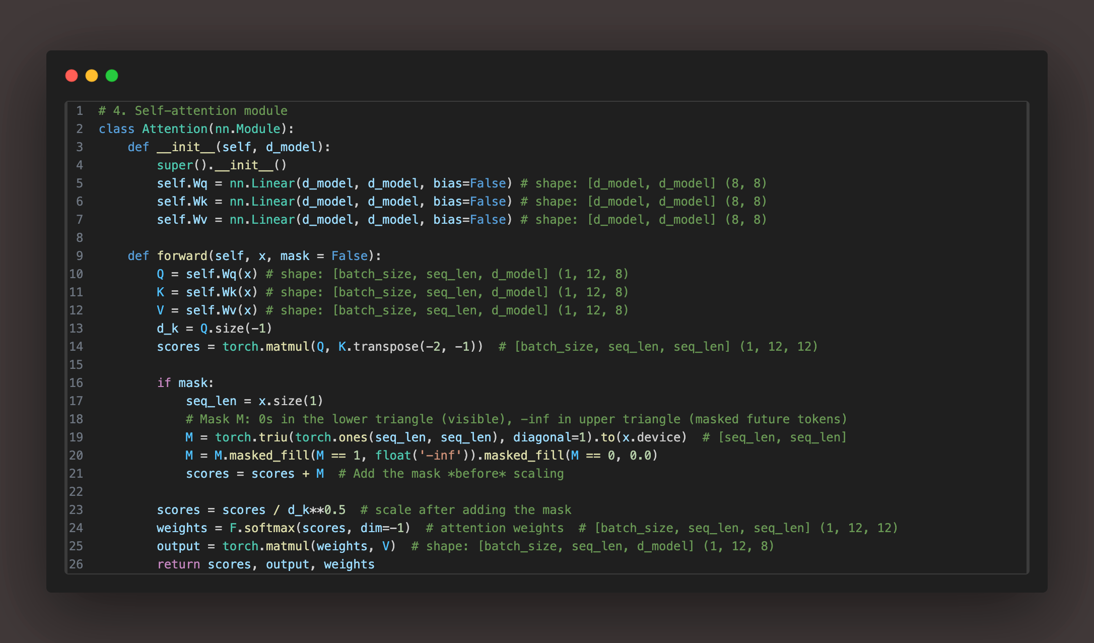
Before we dive further, this is how we usually how self-attention is implemented. Code
Which part of the output is responsible for predicting the next token?
In autoregressive decoding, only the final row (last token’s vector) in the output of the last decoder layer is used to predict the next token. Because the last row encodes all context up to the current token using self-attention. Each earlier row is only used to predict earlier tokens during training — not at inference time.
Visualising the weight matrix without KV Cache
Here is the code to implement self - attention without KV Cache
Let’s try to visualising how the weight matrix changes after projection i.e. the Q, K, V matrix in the self-attention mechanism while going form time t=0 to t=2.
Here is the visualised version of how the Q, K, V projection will look while moving from time stamp 0 to 2.
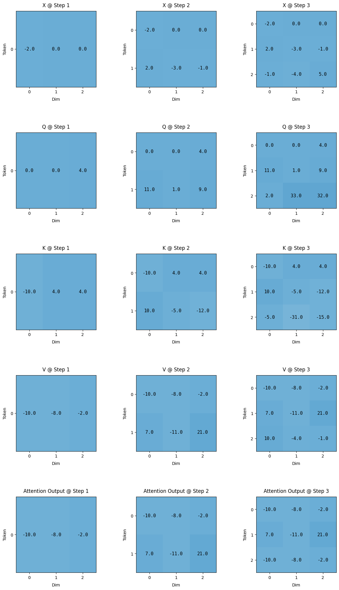
One very important thing to note in here, is that while moving from time = 0 to time = 2, the matrix are getting appended, so the previously step calculated matrix don’t change as we predict the next word. This is where the optimisation lies. If the matrixes are not getting appended any way, instead of calculating the entire Q, K, V matrix. We can just calculate the new row in each matrix, append them to the existing in memory matrixes and carry on. Remember we just need to calculate the last row of the attention output here. We don’t need the previous row to predict the next token.
Visualising the weight matrix with KV Cache
Here is the code which implements KV cache.
And here are the resultant matrix we get after implementing KV Cache.
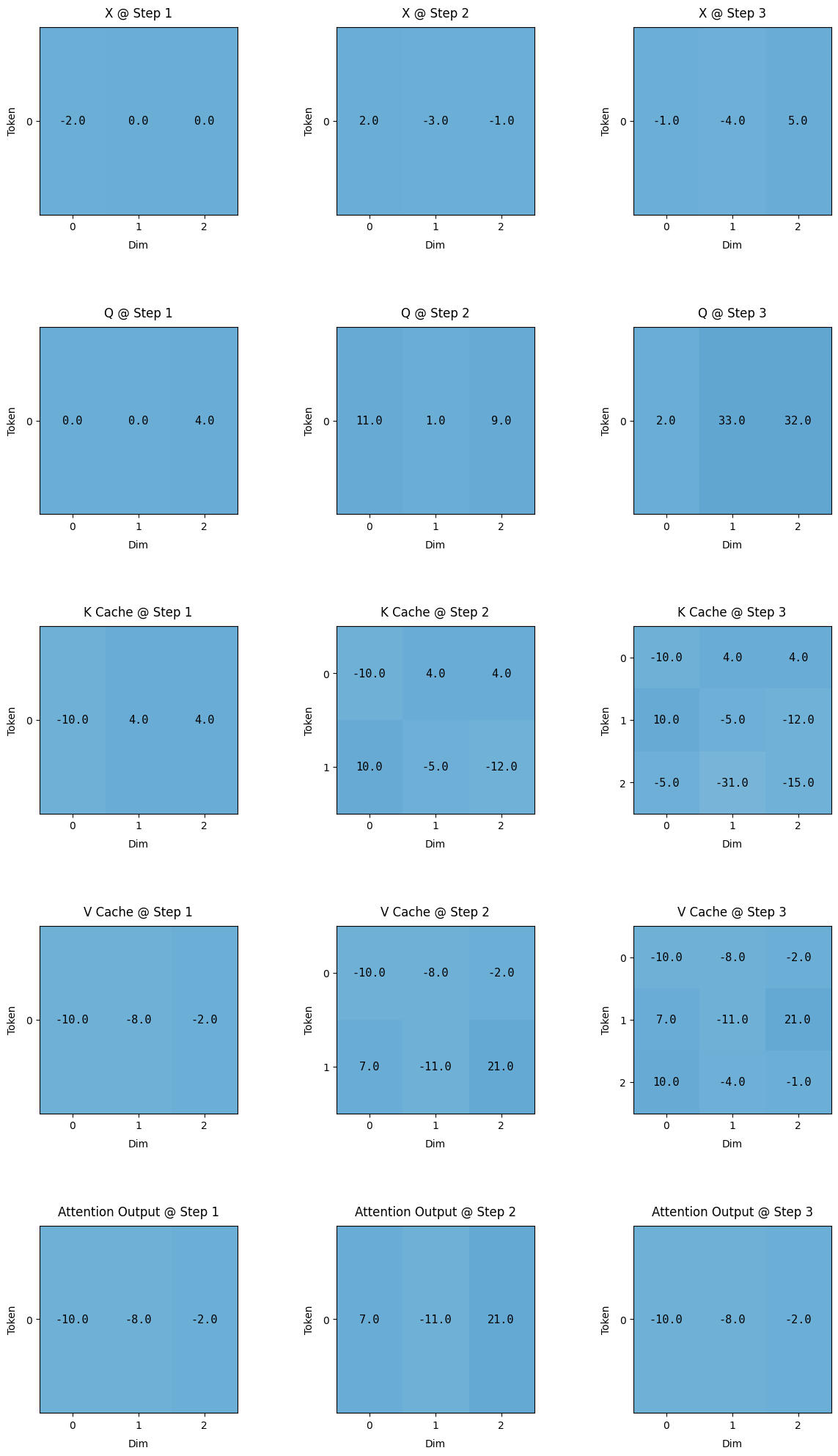
One very important observation is to understand the final row of the attention output, the bottom images at time = 1 and time = 2.
At time = 1, Without KV Cache, the final row is [7.0, -11.0, 21.0] and the same number can be observed with KV Cache [-7.0, -11.0, 21.0]
At time = 2, Without KV Cache, the final row is [-10.0, -8.0, -2.0] and the same number can be observed with KV Cache [-10.0, -8.0, -2.0].
Thus the output doesn’t really get affected with using KV Cache.
Inference time comparison with and without KV Cache
You can find the code for comparison here
Here is the final plot comparing the inference time at each step.
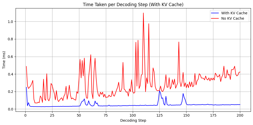
You can clearly see, that with KV caching, the inference time at each step almost remains the same.
Memory required to implement the KV Cache
Well now you have saved a lot of inference time, by saving the weights in Memory. Let’s try to understand the memory requirement we need to implement KV Cache.
I hope you liked the tutorial, here the Github repository containing all the code and images.
Conclusion / Dynamic Programming Relation
Now we know that we can save the weights in memory and then use those weights again in the future. To be honest this is what we do when we try to solve a dynamic programming, there also to save the time we save the sub-part solution in memory which can be referenced later on whenever required.
Thus in my opinion what memoization is to Dynamic Programming, KV Caching is to Transformers. Both are used to save the time and does calculation only once.